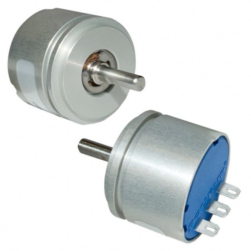
The Bourns Inc. AMS22S5A1BLAFL333, identified by the SKU AMS22S5A1BLAFL333, is a non-contacting rotary position sensor offering a 330-degree electrical angle. This device is designed for robust, long-life applications where precision and durability are paramount. To effectively utilize this component, a thorough interpretation of its datasheet is essential, beginning with its key electrical specifications. The primary output is an analog voltage ratiometric to the supply voltage. The datasheet specifies a supply voltage range, typically 5.0 VDC ± 0.5 VDC. In practice, this means the output voltage at a given angle is directly proportional to the supply voltage. For example, at 5.0V supply, the output will swing from near 0V to near 5.0V over the 330-degree range. If the supply drifts to 5.5V, the output at the same angle will also scale proportionally. The output voltage at the start of the measurement range is typically 0.25V ± 0.05V, while at the end it is 4.75V ± 0.05V, providing a clear, linear signal. The linearity error is a critical parameter, often specified as ±0.5% of the full-scale output. This indicates the maximum deviation from an ideal straight-line transfer function, which is crucial for precise angular measurement. The resolution is essentially infinite due to the analog nature of the Hall-effect sensor, limited only by the noise floor and the resolution of the analog-to-digital converter (ADC) used to read the signal. The output impedance is typically low, often around 2.5 kΩ, allowing it to drive typical ADC inputs directly without significant loading errors.
Understanding absolute maximum ratings is vital for preventing catastrophic failure and ensuring long-term reliability. The datasheet will list maximum supply voltage, output short-circuit duration, and storage temperature range. Exceeding the maximum supply voltage, even momentarily, can permanently damage the internal Hall-effect sensor and signal conditioning circuitry. Derating is a practical consideration for applications near the extremes. For instance, if the ambient temperature exceeds the recommended operating range (typically -40°C to +125°C), the reliability and accuracy may degrade. It is prudent to derate the supply voltage by 5-10% if operating at the upper temperature limit for extended periods. The mechanical specifications are equally important. The shaft loading, both axial and radial, must not exceed the maximum ratings, as this can cause bearing failure or shaft misalignment, leading to erratic output or mechanical seizure. The datasheet will specify a maximum shaft speed, often in the range of 6000 RPM. Operating at higher speeds can cause wear on the sleeve bearing and reduce the sensor's lifespan.
Analyzing a typical application circuit is straightforward for this sensor. The AMS22S5A1BLAFL333 uses a standard three-wire interface: VCC (supply voltage), GND (ground), and VOUT (output voltage). A critical component is a decoupling capacitor, typically 0.1 µF ceramic, placed as close as possible to the VCC and GND pins. This capacitor filters out high-frequency noise on the power supply line, which can couple into the sensitive analog output. The VOUT pin should be connected directly to the ADC input of a microcontroller or dedicated ADC chip. Because the output is ratiometric, the ADC's reference voltage should ideally be the same as the sensor's supply voltage. If the ADC has an independent reference, the system must account for supply variations, either by measuring the actual supply voltage or by using a voltage regulator that is stable over temperature and load. No external pull-up or pull-down resistors are required on the output pin, as it is a low-impedance analog driver. The datasheet may also show a recommended layout for the PCB to minimize noise pickup, often advising a ground plane under the sensor and short, direct traces for the output signal.
The pin configuration is simple: three solder lug terminals, typically labeled 1 (VCC), 2 (GND), and 3 (VOUT). The package is a robust, sealed housing with a 6mm flatted shaft and a bushing mount. The solder lugs are designed for direct wire attachment or soldering to a PCB. The housing material is often plastic with a metal bushing, providing electrical isolation and mechanical strength. For thermal management, the sensor's power dissipation is low, typically less than 50 mW, so active cooling is not required. However, the sensor's accuracy can be affected by self-heating if it is placed near other heat-dissipating components. The datasheet provides a thermal resistance specification, often around 100°C/W. This means for every 0.1W of power dissipated, the internal temperature rises by 10°C above ambient. In practice, this is negligible, but engineers should ensure that the ambient temperature around the sensor does not exceed the rated limit. Mounting the sensor on a metal chassis can help conduct heat away, but this is usually unnecessary given the low power.
Interpreting the timing diagrams and characteristic curves is fundamental. The primary curve is the transfer function: a graph of output voltage versus rotational angle. This is a straight line from the minimum to maximum voltage over the 330-degree range. The datasheet will show this as "Output Voltage vs. Angular Position," typically measured clockwise from a reference point. The slope of this line is the sensitivity, measured in mV/degree. For a 330-degree range and a 4.5V swing (from 0.25V to 4.75V), the sensitivity is approximately 13.6 mV/degree. Any deviation from this straight line is the linearity error. The datasheet may also show a hysteresis curve, though for a non-contacting sensor, hysteresis is typically very low, less than 0.1 degrees. Timing diagrams are less common for analog output sensors, but the datasheet may include a diagram showing the output settling time after a step change in shaft position. This is typically very fast, on the order of microseconds, due to the Hall-effect technology. The response time is dominated by the bandwidth of the internal amplifier and the output driver. The output voltage is stable and does not exhibit significant ripple or noise, but a graph of output noise spectral density may be provided for high-precision applications. The temperature drift curve shows how the output voltage changes with temperature across the range. This is often specified as a percentage of full-scale output per degree Celsius, typically around ±0.05%/°C. Engineers must account for this drift in their system error budget. For example, a 50°C temperature change could introduce a 2.5% error in the output if uncompensated. Software calibration or temperature compensation circuits can mitigate this. By studying these curves and specifications, the engineer can confidently design the AMS22S5A1BLAFL333 into systems requiring reliable, long-life angular position sensing.